Calculations

GLOSSARY

KPI	Key Performance Indicator, also used as a generic term for visualisation components on a dashboard (e.g. Dial, Gauge, Status Indicator etc.)
Tag	An industry term for the name (or ID) of the timeseries data for a sensor in a data historian. All equipment in a facility is “tagged” with a unique identifier, and these unique identifiers are commonly referred to as “tags”.

1 Overview of Calculations

1.1 What are Calculations

Calculations apply “in-line” transforms to any timeseries data source connected to Ingenuity. Anything from simple mathematical operators such as Add, Subtract, Multiply and Divide, through more complex Totalisers and statistical functions like Average and Standard Deviation, logical If..Then functions and complex transforms such as Timeshifting.

Calculations can be nested, and multiple transforms can be applied sequentially.

The output of a Calculation is a Virtual or Synthetic timeseries that can be used in the Ingenuity in exactly the same way other Timeseries sources.

Unlike most of the other modules in Ingenuity, the Calculations module is not shown in the left hand panel because it behaves as a Historian datasource. It is accessible from any component that can take a Historian datasource.

1.2 What are Virtual Timeseries?

Virtual timeseries behave exactly like ‘normal’ (i.e. real or raw) signals stored as tags in process data historians but they are evaluated only when they are called. They can be used in exactly the same way as normal historian tags in Ingenuity.

For example, you can set limits & alerts or use as the basis for another virtual timeseries, but they are evaluated at runtime and do not need the values to be written back to a database.

The advantage of this is that they can be immediately plotted for any time period for which the source data exists, but they do not fill up storage space.

This allows experimentation and quick calculations for analysis without worrying about filling up memory or waiting until historical values are recalculated.

Virtual timeseries can be nested and multiple different functions combined in a single timeseries to produce complex calculations.

1.2.1 Example — unit conversion

If a pressure is measured in ‘bara’ but is required in ‘psia’ then it must be transformed by multiplying it by 14.5. If the source tag is called “Pressure-123” then the calculation would be:

calc/MUL(Pressure-123, 14.5)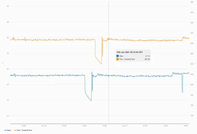

The orange series is a virtual timeseries created by multiplying the original tag (blue) in ‘Bara’ by 14.5 to get ‘Psia’ and then timeshifting the results by 3 hours forwards.

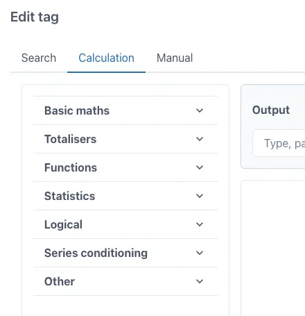
1.3 Creating Calculations (accessing the Editor)

The Calculation graphical editor is on the “Calculation” tab in the “Edit tag” form.

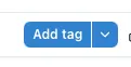
This form appears when the “Add tag” button is clicked on a trend:

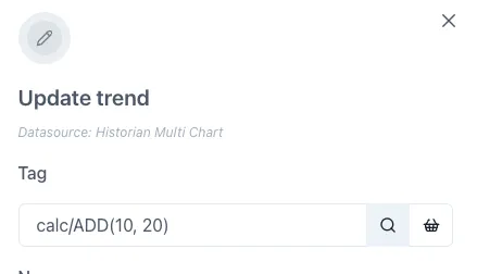
Or when the magnifying glass icon is clicked on the right hand side of the tag datasource entry field when editing a tag on a trend or dashboard:

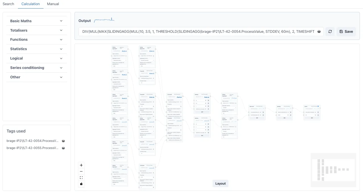
1.4 Editing the Calculation Equations

Ingenuity 7’s virtual calculation graphical editor is an easy-to-use drag-and-drop user interface in which any Ingenuity user can quickly configure complex calculations while minimizing human error.

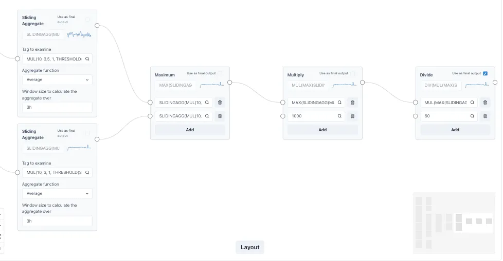
Transform function blocks are dragged and dropped into a canvas, after which inputs and outputs can be connected to compose any complex transformation.

Calculations can be linked together to form complex expressions multiple layers deep and the performance remains fast.

The extract below is from a function that calculates chemical dosing based on tank level changes.

1.5 Example use cases

1.5.1 Smoothing noisy signals

Averages can be applied to smooth out noisy signals

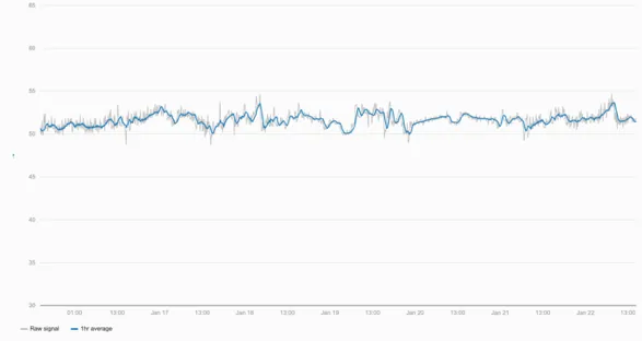
By applying an averaging function with a 1-hour window the underlying trends in the data can be seen more easily.

1.5.2 Logical expressions

The green series in the trend below uses the Threshold function to create a virtual timeseries of the flow only when Pump B is running.

By using a Threshold function to only display the flowrate if the running signal is >0.5, a virtual timeseries is created that could drive a virtual flowmeter graphic.

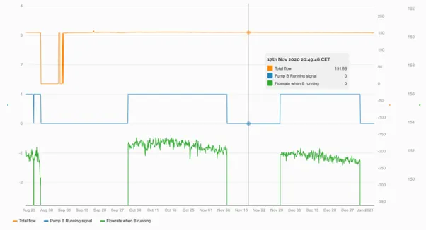
1.5.3 Totaliser

Using the Totaliser function allows a value to be totalised over any window from 1 minute to years.

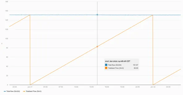
A flowrate in Sm3/d is totalised over 24hrs starting at midnight, giving the cumulative flow so far in any given day (orange line).

1.5.4 Combining two functions

Combining a Totaliser function with a Threshold function we can combine the two examples above to see the total amount of fluid pumped by Pump B in a year.

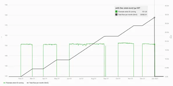
The virtual timeseries of the flow through Pump B is totalised in a second virtual timeseries over a window of a year starting at midnight on the 1^st January.

1.5.5 Taking the Maximum of several tags

The Max function lets users create a virtual timeseries that only shows the maximum value at any time from two or more tags.

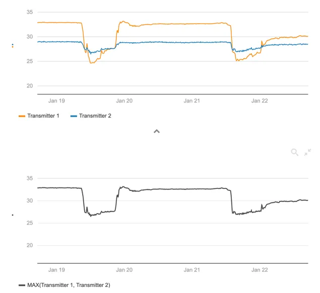
The upper trend shows the readings from two different transmitters. Using the Max function, we are able to create a virtual timeseries (lower trend — black line) that always shows the maximum reading from either of these two transmitters.

2 Calculation Details

2.1 Calculation summary

The table below is a quick reference for all the calculations. All calculations must be preceded by “calc/”, for example calc/ADD(a,b). This prefix will be added automatically by the UI but should be remembered if typing a calculation manually. The placeholders a, b etc. can be a constant value or another timeseries source, or another calculation.

Basic Maths:

Name	Syntax	Notes
Add	ADD(a, b, ..., n)
Subtract	SUB(a, b, ..., n)	Evaluated right to left (n - … - b - a)
Multiply	MUL(a, b, ..., n)
Divide	DIV(a, b)	Evaluated right to left (n / … / b / a)
Percent Deviation	PERCENT(a, b)	Evaluated as 100*(a - b)/b

Totalisers:

Name	Syntax	Notes
Totalise	TOTALISE(a, window, starttime, rate)	See section 0-*
Totalise Raw	TOTALISERAW(a, window, starttime, rate)	See section 2.7.3

Function:

Name	Syntax	Notes
Exponential	EXP(input)	See section 2.8.1
Natural Log	LN(input)	See section 2.8.2
Square Root	sqrt(input)	See section 2.8.3
Log	LOG(input, b)	See section 2.8.4
Power	POWER(input, b)	See section 2.8.5

Sliding Aggregates (normal and raw):

Name	Syntax	Notes
Average	SLIDINGAGG(input, AVG, window)	See section 2.9.1
Count	SLIDINGAGG(input, COUNT, window)	See section 2.9.2
Number of Bad Points	SLIDINGAGG(input, NUMBAD, window)	See section 2.9.3
Number of Good Points	SLIDINGAGG(input, NUMGOOD, window)	See section 2.9.4
Standard Deviation	SLIDINGAGG(input, STDEV, window)	See section 2.9.5
Variance	SLIDINGAGG(input, VAR, window)	See section 2.9.6
Minimum	SLIDINGAGG(input, MIN, window)	See section 2.9.7
Maximum	SLIDINGAGG(input, MAX, window)	See section 2.9.8
Sum	SLIDINGAGG(input, SUM, window)	See section 2.9.9
DIFF	SLIDINGAGG(input, DIFF, window)	See section 2.9.10

Windowed Aggregates:

Name	Syntax	Notes
Same functions as SLIDINGAG	SLIDINGAGG(input, function, window)	See section 2.10

Statistics:

Name	Syntax	Notes
Maximum	MAX(a, b, ..., n)	See section 2.11.1
Minimum	MIN(a, b, ..., n)	See section 2.11.2
Mean	MEAN(a, b, ..., n)	See section 2.11.3
Median	MEDIAN(a, b, ..., n)	See section 2.11.4
Standard Deviation	STDEV(a, b, ..., n)	See section 2.11.5
Variance	VAR(a, b, ..., n)	See section 2.11.6

Logical:

Name	Syntax	Notes
If Tag Exists	IFEXISTS(tag, aIfTrue)	See section 2.12.1
If Equals	IFEQUALS(tag, ifTrue, ifFalse, precision)	See section 2.12.2
Threshold	THRESHOLD(a, b, ifAboveOrEqual, ifBelow)	See section 2.12.3

Series Conditioning:

Name	Syntax	Notes
Stepped	STEPPED(tag)	See section 2.13.1
Stepped Raw	STEPPEDRAW(tag)	See section 2.13.2
No BAD	NOBAD(tag)	See section 2.13.3
Timeshift	TIMESHIFT(tag, offset)	See section 2.13.4

Date:

Name	Syntax	Notes
Epoch_Mx	EPOCH_ISO(tag)	See section 2.14

Other:

Name	Syntax	Notes
Point in Time	POINTINTIME(tag, timeReference)	See section 2.15.1

2.2 Valid timeseries inputs

All calculation functions accept a constant value or any valid timeseries source as an input.

A valid timeseries source in Eigen Ingenuity is anything of the form

historian/id

For example:

enterprise historian:	ip21/21PI1234.val
an open source historian:	influx/kitchen_temp
a calculation:	calc/ADD(15,24,35)
signal generator outputs:	siggen/rand10\~5@3600000
constant values:	value/10

Constant values are a special case in that there is no need to prefix them with “value/” as the system will do that automatically.

2.3 Valid Time Units

Many of the calculation functions accept units of time input. The following are valid in all cases:

s: seconds

m: minutes

h: hours

d: days

w: week

mo: months

y: year

For example:

1 second:	1s
1 minute:	1m or 60s
7 days:	7d or 1w
1 calendar month:	1mo
6 hours:	6h

2.4 Relative Time Expressions

Where a calculation is stated as accepting Relative Time Expressions, both offsets and timestamps can be specified as follows, e.g.

• in 2 days

• 5 days ago

• 2 days and 5 seconds

• in 2 days at the same time

• 2 days and 5 minutes ago

• last moment of yesterday

• in 3 days at midnight*

• now

*forward looking expressions are only relevant if there is data in the future!

The following are not supported:

• Day names: for example it is not valid to say “last moment of last Sunday”.

• Vague time expressions: for example “yesterday at lunchtime”

• Partial day references: for example “morning”

• Holiday names

2.5 RAW vs INTERPOLATED points

In the following descriptions, reference is often made to Raw and Interpolated points.

Raw points are real data points that have been stored in the underlying data historian.

Interpolated points are virtual data points calculated from the raw points.

By default Interpolated points are used in charts and KPIs but the user can change this to Raw points. The reason for this is that the User Interface has no awareness of the number of raw points in a tag before it queries it. If the tag has very high frequency data (for example one point per second) then the returned dataset will be very large and could take a long time to load, or worse, crash the users browser. Conversely, if the underlying tag is very sparse, for example a safety valve position which only moves occasionally, there may be no data within the window requested.

To overcome this issue, Ingenuity 7 will default to 1000[^1] interpolated points on a trend (this can be changed in the trend configuration) to ensure that a trend will always load and then the user can decide to switch to raw points.

2.6 Basic Maths

2.6.1 Add, Subtract, Multiply, Divide

These functions take a list of inputs separated by commas. The syntax for the Basic Maths functions ADD, SUB, MUL and DIV is:

ADD(a, b,..., n)

SUB(a, b,..., n)

MUL(a, b,..., n)

DIV(a, b,..., n)

a, b,.. n — any valid timeseries input (see section 2.2)

The inputs are processed from right to left which means that the SUB and DIV functions will return different results depending on the order of the inputs:

DIV(10, 8) = 1.25

DIV(8, 10) = 0.8

2.6.2 Percent Deviation

This function returns the percent deviation of input b from input a. The syntax for the PERCENTDEV function is:

PERCENTDEV(a, b)

It is evaluated as 100 *(a-b)/b. For example:

PERCENTDEV(10, 8) = 25

PERCENTDEV(8, 10) = -20

2.7 Totalisers

The Totalise functions integrate the area under a trend over the specified window and starting at a specified time. For example, totalising a flow will return the total volume since the start of the window.

The TOTALISE function is the original integral function and has since been superseded by the (backwards compatible) TOTALISE2 function, which is more advanced and better at handling calendar time intervals and daylight savings time.

At some point the TOTALISE algorithm will be replaced by the TOTALISE2 code but any calculations will continue to work.

2.7.1 TOTALISE

The TOTALISE function is the original integral function and sums the area under a trend within the defined Window. TOTALISE does not adjust for uneven time periods or daylight savings.

[It is recommended to use TOTALISE2 for any new calculations.]{.mark}

It will follow the selected interpolation mode on a trend. I.e. if the series is set to INTERPOLATED mode then the Totalise2 calculation will request interpolated points when it is being evaluated. This will result in the fastest performance but may give discrepancies vs raw data

The syntax for the TOTALISE function is:

TOTALISE(input, window, windowAnchor, rate)

• input — any valid timeseries input (see section 2.2)

• window — a window size to totalise over (fixed amount of seconds/minutes/hours/days)

• windowOffsetOrAnchor — where this window should be placed and is as an offset from 00:00:00 GMT

• rate — time unit for underlying tag, if it is m3/s then the time unit is seconds, so you would write “1s”, if m3/h then unit is hours, so you would write “1h” (required to properly scale result)

Window Definition

The Window can be defined as:

• an exact time definition (1s, 12h, 7d, 1w) — see section 2.2

windowAnchor definition

This defines where the start of the totalisation is placed. The options are:

• an offset from 00:00:00 GMT. Negative values shift the start earlier, and positive values shift it later (e.g. -02:00 to align with European summer time - CEST)

  Note: This option will not automatically adjust for daylight savings time when the clocks shift back in the autumn.

• a fixed point in time with optionally specified timezone in the format “YYYY-MM-DD hh:mm:ss ZZZz” (e.g. 2024-04-01 00:00:00 CEST).

  Note: This option is the least efficient as the algorithm will go back to this date every time it is evaluated

2.7.2 TOTALISE2

The Totalise2 function is a newer and more powerful version of the TOTALISE function. At some point the TOTALISE2 logic will replace the TOTALISE logic and they will both work the same way.

The Totalise2 calculation is probably the most used function will follow the selected interpolation mode on a trend. I.e. if the series is set to INTERPOLATED mode then the Totalise2 calculation will request interpolated points when it is being evaluated. This will result in the fastest performance but may give discrepancies vs raw data

The syntax for the TOTALISE2 function is:

TOTALISE2(input, window, windowOffsetOrAnchor, rate)

• input — any valid timeseries input (see section 2.2)

• window — a window size to totalise over (fixed amount of seconds/minutes/hours/days)

• windowOffsetOrAnchor — where this window should be placed this can be specified in four ways; as a pre-defined text expression, as an offset from 00:00:00 GMT, as an expression of time or as a dynamic offset from the current time.

• rate — time unit for underlying tag, if it is m3/s then the time unit is seconds, so you would write “1s”, if m3/h then unit is hours, so you would write “1h” (required to properly scale result)

Window Definition

The Window can be defined as:

• using calendar types: DAY, MONTH, QUARTER, YEAR. These options are pre-defined in the UI

DAY: defaults to midnight of one day to midnight of another

MONTH: defaults to midnight of first day of the month until first day of the next month

QUARTER: defaults to midnight of first day of either january, april, july and October

YEAR: defaults to midnight of 1st of january until begin of next year

• an exact time definition (1s, 7d, 1mo) — see section 2.2

To use this or the following options select “Other” in the Window size definition dropdown:

• by duration definition (PT1S, PT1H, PT24H)

• by period definition (P1D, P1M, P1Y)

• by passing millisecond value (3600000 for 1h)

windowOffsetOrAnchor definition

This defines where the start of the totalisation is placed. The options are:

• Text expressions BEGIN_DAY, BEGIN_MONTH, BEGIN_QUARTER or BEGIN_YEAR will anchor window to the beginning of current period.

  Note: This option is the most popular and will adjust for daylight savings time and the variable length of months

• an offset from 00:00:00 GMT. Negative values shift the start earlier, and positive values shift it later (e.g. -02:00 to align with European summer time - CEST)

  Note: This option will not automatically adjust for daylight savings time when the clocks shift back in the autumn.

• a fixed point in time with optionally specified timezone in the format “YYYY-MM-DD hh:mm:ss ZZZz” (e.g. 2024-04-01 00:00:00 CEST).

  Note: This option is the least efficient as the algorithm will go back to this date every time it is evaluated

• Dynamic offset: Entering a time expression results in the start time of the window being changed dynamically to [now+dynamic offset]. For example, entering ‘0’ means the window is always ending “now”. I.e. it always shows the value of the previous “window” up to now. (This is effectively the same as a SLIGINGAGG(SUM) calculation over the same “window”)
  Entering “-2h” will give the total over the “window” 2 hours ago.

Examples

calc/TOTALISE(tag, YEAR, BEGIN_YEAR, 1h)

will calculate integral since beginning of current year up to current moment.

calc/TOTALISE(tag, MONTH, BEGIN_YEAR, 1h)

will calculate intergral since beginning of current year, starting from 0 at beginning of each month

calc/TOTALISE(1, 1d, 00:00:00, 1h)
= 24 at 23:59:59.999

calc/TOTALISE(1, DAY, BEGIN_DAY, 1d)
= 1 at 23:59:59.999

calc/TOTALISE(1, QUARTER, BEGIN_QUARTER, 1d)
= 90 at 2023-03-31 23:59:59.999
= 91 at 2023-06-30 23:59:59.999
= 92 at 2023-09-30 23:59:59.999
= 92 at 2023-12-31 23:59:59.999

TIP

There are some scenarios where the underlying data needs to be treated as stepped, for example an annual forecast that has a single value for each month at the start of the month. Linearly interpolating between these values will result in errors and so it may be necessary to wrap the tag in a STEPPED() calculation or use TOTALISERAW to make sure that the data is properly interpolated and totalized.

2.7.3 Totalise Raw

The TotaliseRaw function is identical to the Totalise function except that it will force the calculation to use Raw data when it is evaluated, regardless of the Interpolation mode on the trend. This can result in slow performance if there is a lot of data, but it will be very accurate. This might be preferable if the value is to be used in a report.

2.8 Functions

The mathematical functions give access to the common operations for analysing data and evaluating formulae. The EXP, LN and SQRT functions take the form:

fn(input)

input any valid timeseries input (see section 2.2)

The LOG and POWER functions require a second input and the syntax is:

fn(input, b)

input any valid timeseries input (see section 2.2)

b any valid timeseries input (see section 2.2)

2.8.1 EXP: Exponential, e^x

The term “exp(x)” is the same as writing e^x or ℯ^x or “e to the x” or “ℯ to the power of x”. In this context, “ℯ” is a universal constant, ℯ = 2.718281828…

calc/EXP(input)

Example

calc/EXP(10) = 22,026.465...

2.8.2 LN: Natural Log, ln()

The Natural Log is the inverse of the Exponential function. I.e. ln(ℯ^x) = x. The syntax for the LN function is:

calc/LN(input)

Example

calc/LN(5) = 1.609...

calc/LN(EXP(10)) = 10

Important notes

The following should be noted:

• The ln of a negative number is undefined and will throw a “Not a Number” (NaN) error:

• ln(0) is undefined and will throw a “Not a Number” (NaN) error:

• ln(∞)= ∞

• ln(1)=0

• ln(e)=1

• ln(e^x) = x

• e^ln(x)=x

2.8.3 SQRT: Square Root, √x

Square root of a number is a value, which on multiplication by itself, gives the original number. The square root is an inverse method of squaring a number i.e. x². The syntax for the SQRT function is:

calc/SQRT(input)

Example

calc/SQRT(16) = 4

TIP

The square root function is equivalent to raising a number to the power of ½:

SQRT(x) ≡ POW(x,0.5)

2.8.4 LOG: Logarithm Log_y(x)

The Logarithm is the exponent or power to which a base (b) must be raised to return a given number (x).

$${Log}_{b}(x)$$

The syntax for the LOG function is:

calc/LOG(input, b)

input the number for which to find the LOG - any valid timeseries input (see section 2.2)

b the base in which to calculate — any constant or valid timeseries (see section 2.2)

Example

calc/LOG(100,10) = 2

calc/LOG(8,2) = 3

2.8.5 POW: Power, x^y

The POWER function multiplies a number (x) by itself a specified number of times (b). This is often called raising x to the power of b. It is the inverse of the LOG function

$$x^{b}$$

The syntax for the POW function is:

calc/POW(input, b)

input the number to multiply (x) - any valid timeseries input (see section 2.2)

b the power, the number of times to multiply the input by itself— any constant or valid timeseries (see section 2.2)

Example

calc/POW(10,2) = 100

calc/POW(10,-2) = 0.01

calc/POW(2,3) = 8

calc/POW(25,0.5) = 5

2.9 Sliding Aggregates

The SlidingAggregate functions perform an aggregate operation on a single input, over a window. The general construct for SLIDINGAGG functions is:

SLIDINGAGG(input, operation, window)

input — an integer or any valid timeseries source

operation — the short name for one of the operators listed below (AVG, COUNT, NUMGOOD, NUMBAD, STDDEV, VAR, MIN, MAX, SUM, DIFF)

window — any valid time input — see section 2.2

TIP

SLIDINGAGG functions are the most data-hungry calculations and can cause memory problems with either very large window sizes, or, very large time periods with a small window size (e.g. a 2 year trend with a window size of 1hr). If you need to view trends over large periods, consider restructuring the calculation to reduce the number of points the SLIDINGAGG function needs to call.

The function returns the result of the operation over the period of the window immediately preceding the current time. When trending a SLIDINGAGG function, the window is always anchored to beginning of the trend time range.

Example

SLIDINGAGG(input, AVG, window)

Will return a timeseries of the average of the preceding hour at every point in time

The difference between the Sliding Aggregates and the Statistics functions is that the Statistics functions operate across the inputs at each point in time, whereas the Sliding Aggregates operate on a single tag over a window.

2.9.1 AVG: Average

Returns an averaged value of the input over the window. This is an extremely useful function for smoothing out noisy signals. The syntax for a sliding aggregate AVG function is:

SLIDINGAGG(input, AVG, window)

2.9.2 COUNT: Count

Returns the count of the number of points in the window. The syntax for a sliding aggregate COUNT function is:

SLIDINGAGG(input, COUNT, window)

2.9.3 NUMBAD: Number of Bad Points

Returns the count of the number of points with a “bad” status in the window. The syntax for a sliding aggregate NUMBAD function is:

SLIDINGAGG(input, NUMBAD, window)

2.9.4 NUMGOOD: Number of Good Points

Returns the count of the number of points with a “bad” status in the window. The syntax for a sliding aggregate NUMGOOD function is:

SLIDINGAGG(input, NUMGOOD, window)

2.9.5 STDDEV: Standard Deviation

Returns the standard deviation of the data in the window. The syntax for a sliding aggregate STDDEV function is:

SLIDINGAGG(input, STDDEV, window)

2.9.6 VAR: Variance

Returns the variance of the data in the window. The syntax for a sliding aggregate VAR function is:

SLIDINGAGG(input, VAR, window)

2.9.7 MIN: Minimum

Returns the minimum value of the data in the window. The syntax for a sliding aggregate MIN function is:

SLIDINGAGG(input, MIN, window)

2.9.8 MAX: Maximum

Returns the maximum value of the data in the window. The syntax for a sliding aggregate MAX function is:

SLIDINGAGG(input, MAX, window)

2.9.9 SUM: Sum

Returns the sum of all the values of the data in the window. The syntax for a sliding aggregate SUM function is:

SLIDINGAGG(input, SUM, window)

2.9.10 DIFF: Difference

Returns the difference between the last and the first values of the data in the window. The syntax for a sliding aggregate DIFF function is:

SLIDINGAGG(input, DIFF, window)

If the last value is lower than the first value, then the result is negative. This is very useful for calculating gradients.

2.10 Windowed Aggregates

This calculation is an optimized SLIDINGAGG variant that uses historian-provided aggregates to speed up data retrieval time. Instead of calculating over a sliding window, it calculates the aggregates over consecutive fixed windows within the time period.

The syntax of the WINDOWAGG function is:

calc/WINDOWAGG(input, operation, window)

input — an integer or any valid timeseries source

operation — the short name for one of the operators listed below (AVG, COUNT, , NUMBAD, STDDEV, VAR, MIN, MAX, SUM, DIFF)

window — any valid time input — see section 2.2

The available operations for WINDOWAGG are AVG, MIN, MAX, COUNT, STDDEV, VAR. The functions as the same as for the SLIDINGAG calculation.

IMPORTANT NOTES on WINDOWAGG:

[[To achieve best performance, this calc should be used on historian tags, not on other calculations.]{.underline}]{.mark}

• Windows are anchored to closest midnight UTC before requested range.

• When using not “round” window size, windows since day 2 of request will be placed after previous, not after midnight UTC.

• To achieve best performance, this calc should be used on historian tags, not other calcs.

• Aggregates like MIN, MAX and COUNT are stepped (step-after), raw points are generated at beginning of each window.

• Aggregates like AVG, STDDEV, VAR are linearly interpolated, raw points are generated in the middle of each window.

• When requesting interpolated points, window size is increased to match interpolated point interval, when requested window count would be at least twice more than requested interpolated point count. This changes slightly how this calc works, but makes sure that all values in requested area are used, so effectively we query for a continuous time range.

2.11 Statistics

These functions take a list of inputs separated by commas and will return the result of the function across all the inputs at each point in time:

function(a,b,..,n)

The order of the inputs is not important

2.11.1 MAX: Maximum

The minimum of all the inputs at each point in time. The syntax for a MAX function is:

MAX(8,7,4) = 8

2.11.2 MIN: Minimum

The minimum of all the inputs at each point in time. The syntax for a MIN function is:

MIN(8,7,4) = 4

2.11.3 MEAN: Mean

The mean of all the inputs at each point in time. The syntax for a MEAN function is:

MEAN(8,7,4) = 6.33

2.11.4 MEDIAN: Median

The median of all the inputs at each point in time. The syntax for a MEDIAN function is:

MEDIAN(8,7,4) = 7

2.11.5 STDDEV: Standard Deviation

The standard deviate of all the inputs at each point in time. The syntax for a STDDEV function is:

STDDEV(8,6,4) = 2

2.11.6 VARIANCE: Variance

The standard deviate of all the inputs at each point in time. The syntax for a VARIANCE function is:

VARIANCE(8,6,4) = 4

2.12 Logical

The Logical functions allow the user to change the data that is returned depending on if a certain condition is true. They do not apply any mathematical operations on the data.

2.12.1 IFTAGEXISTS: If Tag Exists

This function prevents errors where a valid timeseries does not exist. If a valid dataset is returned then it is returned by the function, otherwise the specified response is provided. The syntax for an IFTAGEXISTS function is:

IFTAGEXISTS(a, ifFalse)

a — a constant or timeseries source to check and return if valid — see section 2.2

ifFalse — a constant or any valid timeseries source to return if (a) is invalid — see section 2.2

2.12.2 IFEQUALS: If Equals** CHANGE WHEN CALC IS UPDATED**

This function compares two inputs (a & b) and returns one timeseries if the result is true (to within the specified precision), otherwise it returns an alternative timeseries. The syntax for an IFEQUALS function is:

IFEQUALS(a, b, ifTrue, ifFalse, <precision>)

a — a constant or any valid timeseries source — see section 2.2

b — a constant or any valid timeseries source — see section 2.2

ifTrue — a constant or any valid timeseries source — see section 2.2

ifFalse — a constant or any valid timeseries source — see section 2.2

precision — OPTIONAL a number specifying the tolerance as either an absolute value or a % tolerance of the average of a & b to apply to the IFEQUALS test. Default = 0.01%.

**CHANGE THIS WHEN CALC IS UPDATED**

In order to keep it simple and make sure that the order of the numbers is not important, the precision is calculated as:

Precision absolute abs\|(a-b)\|

Precision percent abs\|(a-b)/((a+b)/2)\|\*100

i.e. the percentage is the deviation from the average of the two numbers.

TIP

Where an exact deviation is required, for example ±20 against a value of 100, then a precision of 20 should be specified, not 20%.

Important Note

The way the precision percentage is calculated means that the absolute deviation is slightly asymmetric and ranges from a lower percentage for values of b lower than a, and higher for values of b higher than a.

For example, for what range of values of b will the following calculation return 1:

calc/IFEQUALS(100,b,1,0,20%) = 1

This means finding the highest and lowest values of b that make the following expression evaluate to 20:

abs\|(100-b)/((100+b)/2)\|\*100

Evaluating this gives

81.8 \< b \< 122.2

Which ,as a percentage of 100, ranges from 18.2% below up to 22.2% above.

Examples

Using an absolute value of 20 for the precision returns the ifTrue result:

calc/IFEQUALS(80,100,1,0,20) = 1

because the difference is 20:

abs\|(80-100)\|= 20

Using a percentage of 20% as the precision returns the ifFalse value:

calc/IFEQUALS(80,100,1,0,20%) = 0

because the difference is 22.2%:

abs\|(80-100)/((80+100)/2)\|= 20/90 = 22.2%

Use cases

Returning a binary status if a value is within an expected range. For example, a pressure should be 100 ±10%

calc/IFEQUALS(100,PressureReading,1,0,10)

2.12.3 THRESHOLD

This function compares two inputs (a & b) and returns one timeseries a is equal or greater than b, and a different one if it is lower. The syntax for a THRESHOLD function is:

THRESHOLD(a, b, ifaboveorequal, ifbelow)

Example

calc/THRESHOLD(100,50,1,0) = 0

calc/THRESHOLD(100,100,1,0) = 1

calc/THRESHOLD(100,80,1,20) = 20

calc/THRESHOLD(80,100,1,20) = 1

Use cases

Flow masking — return the value of a flowmeter if a valve is open, otherwise return zero. This is useful where a flowmeter does not read exactly zero when there is no flow.

calc/THRESHOLD(ValveStatus,1,FlowReading,0)

Masking out the periods above or below ‘Threshold’.

The function can be used as the filter so the time-series data has ‘gaps’ instead of specific value when the input is above or below the threshold. The following example shows the use case of falling edge detection. When ValveStatus goes from 1 to 0 the function outputs the value = 1 points when the transaction occurs.

calc/THRESHOLD(ValveStatus,1,constants/empty,1)

2.12.4 TIME_THRESHOLD

This function combines the timeseries of two inputs ‘before_tag’ and ‘after_tag’ at the time point specified by ‘timestamp’. The syntax is as follows:

calc/TIME_THRESHOLD(timestamp, before_tag, after_tag)

Use cases

A well designation was changed from producer to injector and a new historian tag was introduced to record wellhead pressure for the new well id. User wishes to visualize the wellhead pressure from the wellbore point of view. To achieve this the two tags can be joined at the point where the designation change occurred.

calc/TIME_THRESHOLD('1-Jan-2022 05:00:00', A21P_WHP, A21I_WHP)

2.13 Series Conditioning

The Series Conditioning functions are used to corrector condition the source data so that it displays correctly in downstream functions.

2.13.1 STEPPED

The Stepped function forces the interpolation algorithm to hold the previous value until a new value is seen. This is essential in the following cases:

• Sparse data that applies for periods of time, for example forecasts; there may be one value per month and it applies for the whole month.

• Binary or discrete data that has not been flagged as stepped in the underlying source*. For example 0 or 1 values, motor running/stopped signals etc. The motor cannot have a state between running and stopped.

* This is a parameters supported by industry standard data historians that identifies a tag as discreet (Boolean, Digital, on/off etc.)

TIP

If tag is configured as stepped in the source, this calc will do nothing and is not necessary.

The syntax for a STEPPED function is:

STEPPED(a)

a — any valid timeseries source — see section 2.2

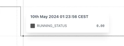
Example

The example below shows that without using the STEPPED function the RUNNING_STATUS shows an implausible value of 0.38 when trended because the underlying tag is not properly configured in the source.

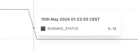
This can be fixed by wrapping the tag in a STEPPED function. Now the change in state properly shown.

2.13.2 STEPPEDRAW: Stepped Raw

The STEPPEDRAW function is identical to the STEPPED function other than it forces the use of Raw data, even if the Trend is set to Interpolated mode.

This is especially useful for reports where one needs to return an accurate total.

Use case

Forcing a TOTALISE calculation to correctly sum a forecast over a month. If the forecast has the following data:

Month	Rate	Monthly Vol.
01-Jan 00:00	1 m3/d	31 m3
01-Feb 00:00	0 m3/d	0 m3

If the Forecast rate is totalised for January without forcing the data to be stepped, then the totalizer will interpolate between 1 and 0 over January and the result will be:

TOTALISE(Rate, MONTH, BEGIN_MONTH, 1d) = 15.5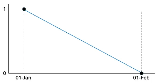

If the Rate is wrapped in a STEPPEDRAW tag it will force the calculation to step the underlying data and the result will be correct.

TOTALISE(STEPPEDRAW(Rate), MONTH, BEGIN_MONTH, 1d) = 31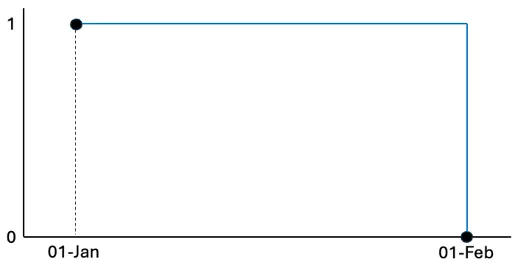

2.13.3 NOBAD: No BAD

The No Bad function removes points from the timeseries that have a “Bad” quality according to the OPC standard[^2] (possible options are Good, Uncertain or Bad) in Raw mode only.

The syntax for a NOBAD function is:

NOBAD(a)

a — any valid timeseries source — see section 2.2

This function has very limited use cases but can help if a tag has randomly incorrect data (i.e. both positive and negative) that cannot be otherwise filtered out.

Because it depends on the raw data, it’s performance can be slower than other functions.

2.13.4 TIMESHIFT

The TIMESHIFT calculation is used when the source data has an incorrect timestamp. This could be because of an incorrectly set timezone or the recording device may have the wrong time. The syntax for a TIMESHIFT function is:

TIMESHIFT(a, offset)

a — any valid timeseries source — see section 2.2

offset — an expression describing how far to shift the data back in time — see below for options

The offset is the amount of time that the source data is away from the time that you want it to be. For example, if a data point is recorded as 06:00 but it should be 07:00 then the data is “1h behind”, so the offset is “-1h” or “-01:00”.

The offset is added to the time range of the data requested so that, if a chart shows data between 12:00 - 14:00 and the TIMESHIFT function has an offset of “1h”, it will return data from the source between 13:00 — 15:00. This has the effect of moving values to the left on a trend. i.e.

Positive values shift data to an earlier point in time.

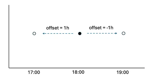
The offset can be defined in several ways. Positive values shift data to an earlier point in time:

• number of milliseconds (3600000 = 1 hour)

• an exact time definition (1s, 1h, 7d etc.) — see section 2.2 Values can be both positive and negative.

• A time expression in hh:mm or hh:mm:ss. For example, to correct a value that is 2minutes and 14 secs slow you would use -00:02:14

•  java-style durations and periods, e.g. P1D for calendar day, PT24H for exactly 24 hours

• relative time expressions, like “2 hours ago” — see section 2.4.

Examples

Retrieve value of tag at end of previous day:

\"calc/TIMESHIFT(calc/TOTALISE2(constants/1, MONTH, BEGIN_MONTH,
1d), **last moment of yesterday**)\",

Retrieve value of tag at end of previous day relative to another date

calc/TIMESHIFT(calc/TOTALISE2(constants/1, MONTH, BEGIN_MONTH, 1d), last
moment of yesterday)\"

2.14 Date

2.14.1 EPOCH_MS: Epoch Milliseconds of raw point

EPOCH_MS Returns number of milliseconds, since 1st January 1970, of each [raw]{.underline} point in the underlying series. For current and historical points it gets last timestamp of point before. i.e for interpolated data it will return the timestamp of the last raw point before.

The syntax for an EPOCH_MS function is:

calc/EPOCH_MS(tag)

Examples

Calculate the number of hours between now and the most recent point stored in the tag:

calc/DIV(SUB(date/CURRENT_EPOCH_MS, calc/EPOCH_MS(tag)),3600000)

This calculation first subtracts the EPOCH_MS of the most recent point from the current time, which will return the number of milliseconds difference. This is then divided by 3,600,000, which is the number of milliseconds in an hour.

2.15 Other

2.15.1 POINTINTIME: Point in Time

The Point In Time function returns that value of the source data at a specific point in time. It is only useful for dashboards and will result in a flat line in a trend. The syntax for POINTINTIME is:

POINTINTIME(a, timereference)

a — any valid timeseries source — see section 2.2

timereference — an expression describing how far to shift the data back in time — see below for options

The timereference can be defined in several ways:

• As an offset from now :

  • number of milliseconds (3600000 = 1 hour)

  • an exact time definition (-1s, -1h, -7d etc.) — see section 2.2

  • relative time expressions, like “2 hours ago” — see section 2.4.

• As a point in time :

  • As a timestamp expression in hh:mm or hh:mm:ss. E.g. 00:00 for midnight this morning

  • relative time expressions, like “last moment of yesterday” — see section 2.4.

Examples

To return the value of a tag at 23:59:59.999 the previous day, the POINTINTTIME syntax is:

POINTINTIME(tag, last moment of yesterday)

Return the value of a tag 2 hours ago:

POINTINTIME(tag, -2h)

2.16 Dates Historian

As of build version ei-v6.71.6 in October 2024 there is a new “Dates” historian that returns data about the date. The available functions in the dates historian are:

dates/CURRENT_EPOCH_MS:

Return current time in epoch ms

dates/IS_TODAY:

Return 1 if given timestamp is today. When trended this will always be zero until the time on the x-axis is today

dates/IS_BEFORE_TODAY:

The opposite of IS_TODAY

dates/DAYS_IN_MONTH:

Returns the number of days in the month of the time requested. When trended this will show a stepped trend of the days in the month for the time on the x-axis

2.17 Signal Generator Historian (siggen)

The Signal Generator or “siggen” historian is built in an is useful for generating example timeseries or for modifying other timeseries (for example the saw wave can be used to convert a daily forecast into a ramp showing the forecast to that point in the day).

The syntax is (without the spaces):

function amplitude +/- y-offset @ period +/- x-offset (in milliseconds)

e.g. sin10-30@600-3600000 — sinewave of amplitude -10 to 10; offset by -30 (i.e. between -40 and -20); with a period of 600 seconds; offset by -3600000 milliseconds (1 hr)

The function will complete one full cycle within the period.

Function supported are:

• sin (sine)

• cos (cosine)

• saw (saw wave) — useful to modify daily values

• sq (square wave) — useful as an on/off signal

• sc (S-curve)

• rand (random) — repeatable random number

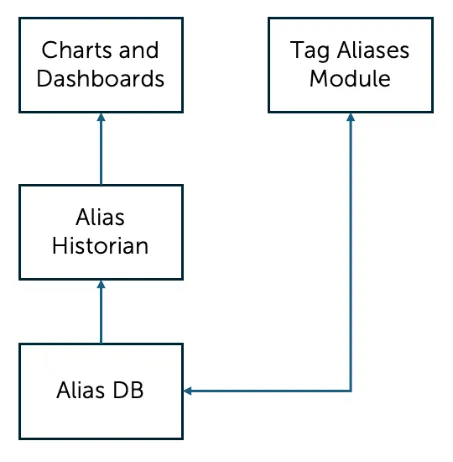
3 The Tag Aliases Module and the Alias Historian

Tag aliases are like nicknames for tags and calculations. The alias name for a tag/calc can be used to search or trend that tag in multiple places The Tag Aliases module is where tag aliases are created and managed and the Alias Historian is the data source that makes them available to charts and dashboards.

3.1 Overview

Tag Aliases are created and managed in the Tag Aliases module. They are stored in a database and made available to use in Charts & Dashboards by the Alias Historian:

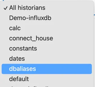
3.2 Using Alias tags

Tag aliases can be searched for in the same way as any other tags. The search can be restricted to only search the Alias Historian by selecting the “dbaliases” data source from the dropdown:

3.3 Accessing the Alias Module

The Tag Aliases is accessed by clicking “Tag Aliases” item in the left hand navigation panel:

The panel on the right shows a pagninated table with all the configured aliases.

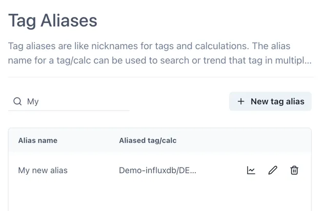
3.4 Creating an alias

To create a new Tag Alias, click the [+ New tag alias] button at the top right. Enter the tag name or calculation in the Tag field (in the usual format of datasource/tagname) and the alias name you would like to use in the “Tag alias name” field.

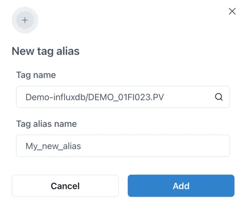
Note: it is good practice not to have spaces in the Tag alias name.

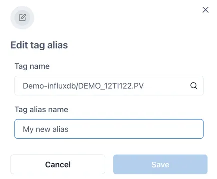
3.5 Editing a Tag Alias

To edit a Tag Alias, click on the edit icon (pencil) at the right hand side of a tag alias to edit it.

Make any changes and then click “Save”.

3.6 Deleting an alias

To delete a Tag Alias, click on the delete icon (dustbin) at the right hand side of a tag alias.

A confirmation pop up appears. Click “Delete” to permenantly delete the tag alias.

4 Working with Calculations

This chapter covers detailed aspects of working with calculations to make more intuitive and user friendly content.

4.1 SLIDINGAGG vs WINDOWAGG

Both SLIDINGAGG and WINDOWAGG are types of aggregate calculations that can be performed on time series data and are used to compute aggregate functions like min, max, average, etc. There are important differences between them though, and these are described below.

Tip

SLIDINGAGG provides a moving aggregation based on a time window over interpolated points, suitable for real-time trends, while WINDOWAGG provides aggregations over fixed time windows, retrieved directly from the historian, and is generally more appropriate for retrospective analysis.

4.1.1 Differences

Data Source for Calculation:

SLIDINGAGG calculations are performed over interpolated points retrieved from the historian . The system retrieves a range of points and then calculates the aggregate over a sliding window.

WINDOWAGG calculations, in contrast, request the aggregated data directly from the historian . If the underlying historian does not support direct aggregate retrieval for the specified window, the Eigen historian driver will simulate it by fetching raw data and performing the aggregation .

Window Behavior:

SLIDINGAGG operates with windows that slide over time1 … For each point in time, the aggregate is calculated based on the data within the preceding (or centered) time window that moves with the current time.

WINDOWAGG uses fixed windows that are aligned to specific time boundaries, anchored to the nearest midnight UTC. The aggregate is calculated for these discrete, non-overlapping time intervals .

Real-time vs. Retrospective Analysis:

SLIDINGAGG provides a consistent view of the aggregated data in both real-time and when looking back at historical data because the calculation is always based on a defined sliding window of past data.

WINDOWAGG can exhibit different behavior in real-time for the current, incomplete, window compared to its retrospective view once the window has fully elapsed. Until the end of the window, the aggregate value (like maximum for a totalizer) will not reflect the full range of data within that window. Therefore, WINDOWAGG is considered more of a retrospective function12 .

Performance:

WINDOWAGG is generally more performant than SLIDINGAGG when the historian natively supports aggregate queries, as it reduces the amount of data that needs to be transferred and computed.

Handling of Peaks:

In SLIDINGAGG, a peak value within the sliding window will influence the aggregate output for the entire duration the peak remains within that window (i.e. from the timestamp of the peak to the timestamp + window).

In WINDOWAGG, a transient peak occurring late in a window might only affect the aggregate calculation for that window briefly in real-time. However, when viewed retrospectively, that peak will be reflected in the aggregate for the entire window. For example, a peak occurring in the 59th minute of a 1 hour window for a MAX calculation will affect the current value for 1 minute but then the whole prior window will take on that value as soon as the window period rolls over to a new one.

Use Cases:

SLIDINGAGG is suitable for applications where a continuously updating aggregate value based on a recent time window is required, such as dashboards showing real-time trends.

WINDOWAGG is well-suited for analyzing data over completed, fixed time intervals, like calculating daily, monthly, or yearly averages, or for visualizing the range (min/max) of values within those fixed periods.

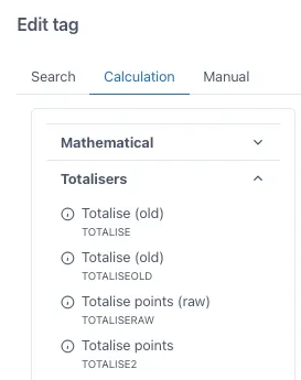
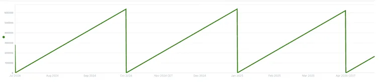
4.2 Calculation example: Totalise for quarterly rates.

In this calculation example we will cover a very popular function from our calculation engine which is Totalise points. For calculating daily rates from a tag with hourly rates, for example, m3/h of production, we have to use the Totalise points function. Drag this function into the grid from the menu in the “Calculation” tab when adding a tag, you will find it under the “Totalisers” tab.

The input to this function will look as follows.

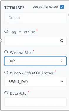
Under “Tag to Totalise” you will add the tag or calculation you wish to totalise. You can click on the magnifying glass to search for a tag if necessary. The tag should have the name of the historian followed by a ”/” before the name of the tag, if you search for it with the magnifying glass there is no need for this. Take note of the units of the tag since we will need this information later.

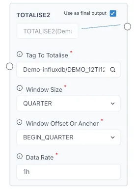
The “Window size” refers to the time span that you wish to totalise your tag to, for example, we have our production tag in m3/h and we wish to know how much we produce per quarter, then the “Window size” should be “Quarter”. Click on it to open the drop-down menu and select the desired option.

For “Window Offset or Anchor” we will select “BEGIN_QUARTER”, this means that it will start from 0 each quarter (1^st January, 1^st April, 1^st July and 1^st October). And lastly, we will add the “Data Rate” from our tag, since this example has a tag with m3/h, the data rate will be “1h” for 1 hour. For 1 second the value would be “1s”, for daily rates it would be “1d”, etc. Here is the input from our example and how it looks on a chart.

5 Common errors and how to avoid them

The following chapter contains recommendations for improving the performance of calculations and avoiding errors.

5.1 Point limit errors.

Trending a calculation over a large time period can result in a point limit error such as:

This SLIDINGAGG request needs to retrieve 52,560 points, but limit is 30000. Try reducing requested range or increasing sliding window size. Reason is that to keep results precise, SLIDINGAGG retrieves at least 3 points for each window that fit in requested range.

This is a consequence of how SLIDINGAGG works when retrieving interpolated points. To calculate number of points requested, the whole range is divided by window size and then multiplied by 3, to have at least 3 points in each window to calculate window aggregate. In the case of a trend over 2 years with a window size of 1 hour (i.e. hourly averages) the request is 365*2*24*3 = 52,560.

For more information, please contact us at info@eigen.co or book a demo on our website at www.eigen.co